Coil Current

Now that we've looked at a few coil geometries, let's take a step back. I started FEMM modelling with an important assumption. Is it true that force scales neatly with coil current?

The answer to this question will suggest if there's an advantage to an extremely high magnetic impulse or not. It tells us whether to pursue kilo-volt capacitors, or to build many stages of modest capacitor banks.

FEMM Model

A reader once suggested that exciting things happen when you discharge capacitors above 500v or so. I want to find out if it's as good as they think.

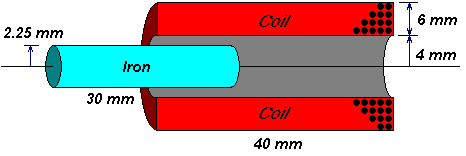
This model approximates my actual parts, using nice round numbers:

• 40mm long coil
• 8mm inside diameter (4mm radius)
• 20mm outside diameter (10mm radius)
• 16 AWG wire (1.29mm diameter)
• An inductor simulation suggests this has 4 layers of 31 turns (51 microhenries, 71 milliohms)

The projectile is made of iron welding rod:

• 4.5mm diameter (2.25mm radius)
• 30mm long (make it 25% shorter than coil)
• M-19 steel (not sure if this is correct, but it matches my other FEMM models)
• air gap is practically filled with a plastic firing tube (not shown)

Like my other FEMM models, this model has some important assumptions:

• frequency is d.c. (no eddy currents)
• velocity is zero (every point is simulated at steady-state with no motion)
• projectile is M-19 steel (nonlinear BH curve)
• steady coil current (not a capacitive-discharge system)
• no losses due to friction (don't we wish!)

FEMM Coil Current

We'll use Lua scripting to explore a range of coil currents from 10 - 10,000 amps. This is a wider range than I need -- I expect my actual coilgun's peak current to fall somewhere above a mere 100 amps. But we're interested to see what happens at really high current.

FEMM accepts "current" as a sheet density. Here's how to convert wire current w to coil current c. First compute amp-turns:

N*I = (layers)*(turns)*(current) = 4 * 31 * w

Next compute cross-sectional area of coil windings:

Area = (outer radius - inner radius)*(coil length)
Area = (10mm - 4mm)*(40mm) = 240mm²

Finally compute current density:

J = (amp-turns)/(area) = 124w / (240mm²) * (10⁶ mm² per m²)
J = 0.516667w mega-amps per m²

This equation will be used in the Lua script below.

Pre-processor Lua Program

outfile = "coilcurrent_results.txt"
handle=openfile(outfile,"a")
write(handle, "\nComparing various coil currents\n")
write(handle, "      from 100 amps to 10,000 amps\n")
write(handle, "Coil is 40mm long\n")
write(handle, "      4mm inside radius\n")
write(handle, "      10mm outside radius\n")
write(handle, "      4 layers of 31 turns each\n")
write(handle, "Projectile is 30mm long\n")
write(handle, "      2.25mm radius\n")
write(handle, "      made of M-19 steel\n")
write(handle, "      starting 48mm away from center\n")
write(handle, "To import in Excel:\n")
write(handle, "      Data - Get External Data - Import text file\n")
write(handle, "      then choose the file written by this program\n")
write(handle, "      and click Finish.\n")
write(handle, "This data file is tab delimited\n")
write(handle, "      (Excel's default import format)\n")
closefile(handle)

save_femm_file("temp.fem")
seteditmode("group")

increment = 1000

for i=0,11 do
	current = 100 + (i * increment)
	current_density = current * 0.516667
	modify_material("Copper", 4, current_density)

	handle=openfile(outfile,"a")
	write(handle, "\nCoil current = ", current, " amps\n")
	write(handle, "Current density = ", current_density, "MA/m2\n\n")
	closefile(handle)

	for n=1,48 do
		showmesh()
		analyse()

		handle=openfile(outfile,"a")
		write(handle, n-49, "\t")
		closefile(handle)
		runpost("coilcurrent_post.lua")

		selectgroup(1)
		move_translate(0,-1)
	end

	selectgroup(1)
	move_translate(0,48)
end

        

Post-processor Lua Program

groupselectblock(2)
force=blockintegral(12)

handle=openfile("coilcurrent_results.txt","a")
write(handle, force, "\n")
closefile(handle)

exitpost()

        

Results

You can see the detailed Excel spreadsheet here. You can get the raw results file here as it was written by FEMM. For each coil, it computes the force on the projectile at many positions and sums the result.

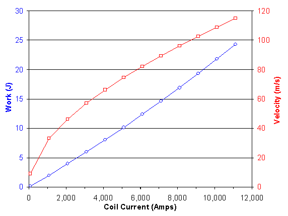
This is a numerical solution to integrating force as it acts over a distance, yielding "work". We ignore friction and losses, and assume the work is converted completely into kinetic energy.The graph shows the total work done for the given continuous coil current.

Conclusion

The graph shows how much kinetic energy (blue) is absorbed by the projectile from various coil currents. It also shows the final velocity (red), assuming that KE = 1/2 * m * v².

The kinetic energy graph is practically a straight line.

The energy transfer is not very sensitive to coil current. This is surprising, since I expected the magnetic saturation to reduce the efficiency with large current.

The result is surprising enough that I tend to discount the outcome. For now, I assume there is a flaw in the modelling procedure.

The modelling should be repeated with a close eye to saturation. The next model should review the ferrous material and check that the B-H curve accurately represents the material at very high magnetic fields. It probably needs adjustment, since FEM warns of accuracy errors if your B-H curve does not include your operating region. The next model should run some tests manually so the amount of saturation can be examined and reviewed. This will tell you where the expected curve should depart from linearity.

The bottom line... There is more modelling and analysis needed here. Comments and suggestions are welcomed.